On fast integer multiplication
Part 0: an incredibly great choice of modulus
The standard approach for multiplying two integers requires incredibly large prime modulus, to facilitate the convolution of sequences of relatively large integers. For this purpose we choose $p=2^{64}-2^{32}+1$, the benefits of which are described by Adam P. Goucher.
How would we quickly number theoretic transform modulo $p$?
Part 1: fast reduction
Suppose we have some 64-bit nonnegative integer $x=A2^{96}+B2^{64}+C$ which we desire to reduce modulo $p$, where $A,C<2^{64}$ and $B<2^{32}$. As $2^{96}\equiv -1\pmod p$ and $2^{64}\equiv 2^{32}-1\pmod p$, reduction is implementable without the usage of any 128-bit operations.
constexpr uint64_t p = 1 - (1ull << 32);
uint64_t re(uint64_t A, uint64_t B, uint64_t C) {
  uint64_t i = C - A + (A > C ? p : 0);
  uint64_t j = (B << 32) - B;
  return i + j - (i >= p - j ? p : 0);
}
Part 2: fast multiplication by powers of 2
One would ask why it is necessary to choose $x$ in the range of $2^{160}$. This facilitates modular bit shifts of all powers of $2$ without 128-bit operations. In particular, suppose we wish to find $x2^{96a+b}$; by our previous observation, this is equivalent to $x(-1)^a2^b$, which is trivially computable with bitwise operations.
In fact, $2$ is a $192$nd root of unity of $p$; this particular characteristic of $p$ makes mixed-radix magic possible.
uint64_t x2k(uint64_t x, int e) {
  int a = e / 96, b = e - a * 96;
  x = (a % 2 ? p - x : x);
  if (!b)
    return x;
  uint64_t A = b < 64 ? x << b : 0;
  uint32_t B = b < 64 ? x >> 64 - b : x << b - 64;
  uint64_t C = b > 32 ? x >> 96 - b : 0;
  return re(A, B, C);
}
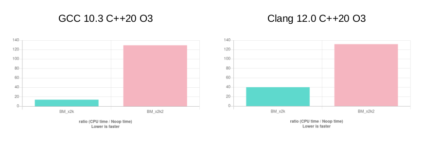
Surprisingly, even though Clang optimizes x2k into branchless code, it is about 3 times slower than the branching code GCC produces. The function x2k2 is standard 128-bit multiplication, provided for comparison.
#include <benchmark/benchmark.h>

constexpr uint64_t p = 1 - (1ull << 32);
uint64_t re(uint64_t A, uint64_t B, uint64_t C) {
  uint64_t i = C - A + (A > C ? p : 0);
  uint64_t j = (B << 32) - B;
  return i + j - (i >= p - j ? p : 0);
}
uint64_t x2k(uint64_t x, int e) {
  int a = e / 96, b = e - a * 96;
  x = (a % 2 ? p - x : x);
  if (!b)
    return x;
  uint64_t C = b < 64 ? x << b : 0;
  uint32_t B = b > 64 ? x << (b - 64) : x >> (64 - b);
  uint64_t A = b > 32 ? x >> (96 - b) : 0;
  return re(A, B, C);
}
uint64_t x2k2(uint64_t x, int e) {
  int a = e / 96, b = e - a * 96;
  x = (a % 2 ? p - x : x);
  __uint128_t s = 1;
  s <<= b;
  s %= p;
  return x * s % p;
}

static void BM_x2k(benchmark::State &state) {
  // Perform setup here
  uint64_t x = 0;
  int e = 0;
  volatile uint64_t tt = 0;
  for (auto _ : state) {
    // This code gets timed
    x++;
    e++;
    tt += x2k(x, e);
  }
}

static void BM_x2k2(benchmark::State &state) {
  // Perform setup here
  uint64_t x = 0;
  int e = 0;
  volatile uint64_t tt = 0;
  for (auto _ : state) {
    // This code gets timed
    x++;
    e++;
    tt += x2k2(x, e);
  }
}
// Register the function as a benchmark
BENCHMARK(BM_x2k);
BENCHMARK(BM_x2k2);
Part 3: mixed-radix NTT
To use this property - and its according 9.2x speedup over 128-bit multiplication - to its full extent, we need to somehow employ mostly powers of $2$ as roots of unity during the number theoretic transform. Clearly, standard Cooley-Tukey is not going to cut it.
Recall the definition of the NTT:
$$\operatorname{NTT}(a_0,a_1,a_2,\dots,a_{2^n-1})[i]\equiv\sum_{j=0}^{2^n-1}\omega_{2^n}^{ij}a_j\pmod p$$
Standard Cooley-Tukey is effectively an expansion of $j$ into its quotient and remainder modulo $2$. Let’s instead expand $i$ into its quotient and remainder modulo $2$:
For even $i$, we have:
$$\begin{align*}\operatorname{NTT}(\{a_s\}_{s=0}^{2^n-1})[2i+0] & \equiv\sum_{j_0=0}^{1}\sum_{j_1=0}^{2^{n-1}-1}\omega_{2^n}^{(2i)(2^{n-1}j_0+j_1)}a_{2^{n-1}j_0+j_1}\\ & \equiv\sum_{j_0=0}^{1}\sum_{j_1=0}^{2^{n-1}-1}\omega_{2^n}^{2ij_1}a_{2^{n-1}j_0+j_1}\\ & \equiv\sum_{j_1=0}^{2^{n-1}-1}\omega_{2^{n-1}}^{ij_1}\sum_{j_0=0}^{1}a_{2^{n-1}j_0+j_1}\\ & \equiv\operatorname{NTT}(\{a_s+a_{2^{n-1}+s}\}_{s=0}^{2^{n-1}-1})[i]\end{align*}$$
For odd $i$, we have:
$$\begin{align*}\operatorname{NTT}(\{a_s\}_{s=0}^{2^n-1})[2i+1] & \equiv\sum_{j_0=0}^{1}\sum_{j_1=0}^{2^{n-1}-1}\omega_{2^n}^{(2i+1)(2^{n-1}j_0+j_1)}a_{2^{n-1}j_0+j_1}\\ & \equiv\sum_{j_0=0}^{1}\sum_{j_1=0}^{2^{n-1}-1}\omega_{2^n}^{2ij_1+(2^{n-1}j_0+j_1)}a_{2^{n-1}j_0+j_1}\\ & \equiv\sum_{j_1=0}^{2^{n-1}-1}\omega_{2^{n-1}}^{ij_1}\sum_{j_0=0}^{1}(-1)^{j_0}\omega_{2^n}^{j_1}a_{2^{n-1}j_0+j_1}\\ & \equiv\operatorname{NTT}(\{\omega_{2^n}^s(a_s-a_{2^{n-1}+s})\}_{s=0}^{2^{n-1}-1})[i]\end{align*}$$
This method is a bit different from the conventional definition:
$$\operatorname{NTT}(\{a_s\}_{s=0}^{2^n-1})[i]\equiv \sum_{j_1=0}^1\omega_{2^n}^{ij_1}\operatorname{NTT}(\{a_{2j_0+j_1}\}_{j_0=0}^{2^{n-1}-1})[i\bmod 2^{n-1}]$$
This method has the advantage of skipping over the cache inefficient bit reversal part. In fact, the experienced reader will quickly spot that this is oddly similar to the conventional definition of the inverse NTT, derived by inverting the order and butterfly $\begin{bmatrix}x & y\end{bmatrix}\leftarrow \begin{bmatrix}x+\omega y & x-\omega y\end{bmatrix}$:
$$\begin{align*}\operatorname{iNTT}(\{a_s\}_{s=0}^{2^n-1})[2i+0] & \equiv \operatorname{iNTT}(\{\frac{a_s+a_{s+2^{n-1}}}{2}\}_{s=0}^{2^{n-1}-1})[i]\\ \operatorname{iNTT}(\{a_s\}_{s=0}^{2^n-1})[2i+1]&\equiv \operatorname{iNTT}(\{\omega_{2^n}^{-s}\frac{a_s-a_{s+2^{n-1}}}{2}\}_{s=0}^{2^{n-1}-1})[i]\end{align*}$$
This similarity owns to a duality between the normal and inverse transforms:
$$\operatorname{iNTT}(\{a_s\}_{s=0}^{2^n-1}) \equiv \frac{1}{2^n}\operatorname{NTT}(\{a_{(2^n-s)\bmod 2^n}\}_{s=0}^{2^n-1})$$
Thus, we can create a different method for NTT by taking the conventional transform, removing the parts dividing by $2$, effectively multiplying through by $2^n$, and replacing $\omega_{2^n}^{-s}$ with $\omega_{2^n}^s$, effectively reversing the indices of $a$ modulo $2^n$. This is method described above.
If, in a conventional NTT, we need to apply the bit reversal at the beginning, then in a conventional iNTT, we need to apply the bit reversal at the end. This implies that in our new NTT, we need to apply the bit reversal at the end, and in our new iNTT, we need to apply the bit reversal at the beginning. But two bit reversals cancel out, and during convolution all we do is take a dot product, which is order-agnostic; in this way we do away with bit reversal entirely.
One transform of length $2^n$ is decomposed into two transforms of length $2^{n-1}$ in $2^{n-1}$ multiplications, completing the transform in $n2^{n-1}$ multiplications. However, this choice of “two transforms” is rather arbitrary. Let us split it instead into $2^B$ transforms of length $2^{n-B}$:
$$\begin{align*}\operatorname{NTT}(\{a_s\}_{s=0}^{2^n-1})[2^Bi_0+i_1] & \equiv\sum_{j_0=0}^{2^B-1}\sum_{j_1=0}^{2^{n-B}-1}\omega_{2^n}^{(2^Bi_0+i_1)(2^{n-B}j_0+j_1)}a_{2^{n-B}j_0+j_1}\\ & \equiv\sum_{j_0=0}^{2^B-1}\sum_{j_1=0}^{2^{n-B}-1}\omega_{2^{n-B}}^{i_0j_1}\omega_{2^B}^{i_1j_0}\omega_{2^n}^{i_1j_1}a_{2^{n-B}j_0+j_1}\\ & \equiv\operatorname{NTT}(\{\sum_{j_0=0}^{2^B-1}\omega_{2^B}^{i_1j_0}\omega_{2^n}^{i_1s}a_{2^{n-B}j_0+s}\}_{s=0}^{2^{n-B}-1})[i_0]\\ & \equiv\operatorname{NTT}(\{\omega_{2^n}^{i_1s}\operatorname{NTT}(\{a_{2^{n-B}t+s}\}_{t=0}^{2^B-1})[i_1]\}_{s=0}^{2^{n-B}-1})[i_0]\end{align*}$$
For a given $\operatorname{NTT}$ of length $2^n$, the outer $\operatorname{NTT}$ of length $2^{n-B}$ is computed $2^B$ times; once for each $i_1$ from $0$ to $2^B-1$. The inner $\operatorname{NTT}$ of length $2^B$ is computed $2^{n-B}$ times; once for each $s$ from $0$ to $2^{n-B}-1$.
One may intuitively consider this as a two-dimensional NTT on a rectangle of sorts, first over rows, then over columns, with twiddle factors in between. This procedure is aesthetically symmetric. Remember: $2$ is a $192$nd root of unity; choosing $B=6$, upon which we may calculate the inner $\operatorname{NTT}$ using exclusively shifts by powers of $2$.
Part 4: inner NTT
Following benchmarks will be run on a two-core Intel(R) Xeon(R) Gold 6148 CPU @ 2.40GHz cloud compute instance, with 32 KiB, 4 MiB, and 27.5 MiB L1d, L2, and unified L3 cache, respectively.
One may try to directly implement the inner transform like so:
void ntt_inner_1(uint64_t *a, int n = 6) {
  assert(n <= 6);
  int l = 1 << n;
  int p = 192 >> n;
  for (int i = n - 1; i >= 0; i--) {
    for (int j = 0; j < l; j += (2 << i))
      for (int k = 0; k < (1 << i); k++) {
        uint64_t x = sub(a[j + k], a[j + k + (1 << i)]);
        a[j + k] = add(a[j + k], a[j + k + (1 << i)]);
        a[j + k + (1 << i)] = x2k(x, p * k);
      }
    p *= 2;
  }
}
This runs at approximately 4.4μs per call, and is only a modest 3x improvement over the implementation which uses naive multiplication; we can do better. Firstly, observe that $p$ is $192/2^{i+1}$, and $k$ is at most $2^{i}-1$, so $pk<96$. Thus it would be beneficial to do away with x2k entirely and specialize for how the exponent is less than $96$:
void ntt_inner_2(uint64_t *a, int n = 6) {
  assert(n <= 6);
  int l = 1 << n;
  int p = 192 >> n;
  for (int i = n - 1; i >= 0; i--) {
    for (int j = 0; j < l; j += (2 << i))
      for (int k = 0; k < (1 << i); k++) {
        uint64_t x = sub(a[j + k], a[j + k + (1 << i)]);
        a[j + k] = add(a[j + k], a[j + k + (1 << i)]);
        if (!k)
          a[j + k + (1 << i)] = x;
        else {
          int b = p * k;
          uint64_t C = b < 64 ? x << b : 0;
          uint32_t B = b > 64 ? x << (b - 64) : x >> (64 - b);
          uint64_t A = b > 32 ? x >> (96 - b) : 0;
          a[j + k + (1 << i)] = re(A, B, C);
        }
      }
    p *= 2;
  }
}
This optimizes it to 3.5μs per call. Observe that the DFT of length 4 can be calculated in 4 butterflies, only one of which requires a non-trivial multiplication:
$$\begin{matrix} & a & b & c & d\\ \stackrel{\text{(0,2)}}{\Rightarrow} & a+c & b & a-c & d\\ \stackrel{\text{(1,3)}\times i}{\Rightarrow} & a+c & b+d & a-c & ib-id\\ \stackrel{\text{(2,3)}}{\Rightarrow} & a+c & b+d & a+ib-c-id & a-ib-c+id\\ \stackrel{\text{(0,1)}}{\Rightarrow} & a+b+c+d & a-b+c-d & a+ib-c-id & a-ib-c+id \end{matrix}$$
While we’re at it, let’s unroll the branching, and add special reductions for A=0 or C=0, too:
void ntt_inner_3(uint64_t *a, int n = 6) {
  assert(n <= 6);
  if (n == 0)
    return;
  if (n == 1) {
    uint64_t x = a[1];
    a[1] = sub(a[0], x);
    a[0] = add(a[0], x);
    return;
  }
  int l = 1 << n;
  int p = 192 >> n;
  for (int i = n - 1, s = 6 - n; i >= 2; i--, s++) {
    for (int j = 0; j < l; j += (2 << i)) {
      {
        uint64_t x = sub(a[j], a[j + (1 << i)]);
        a[j] = add(a[j], a[j + (1 << i)]);
        a[j + (1 << i)] = x;
      }
      int k = 1;
      for (; k <= (10 >> s); k++) {
        uint64_t x = sub(a[j + k], a[j + k + (1 << i)]);
        a[j + k] = add(a[j + k], a[j + k + (1 << i)]);
        int b = p * k;
        uint64_t C = x << b;
        uint32_t B = x >> (64 - b);
        a[j + k + (1 << i)] = reBC(B, C);
      }
      for (; k <= (21 >> s); k++) {
        uint64_t x = sub(a[j + k], a[j + k + (1 << i)]);
        a[j + k] = add(a[j + k], a[j + k + (1 << i)]);
        int b = p * k;
        uint64_t C = x << b;
        uint32_t B = x >> (64 - b);
        uint64_t A = x >> (96 - b);
        a[j + k + (1 << i)] = re(A, B, C);
      }
      for (; k < (32 >> s); k++) {
        uint64_t x = sub(a[j + k], a[j + k + (1 << i)]);
        a[j + k] = add(a[j + k], a[j + k + (1 << i)]);
        int b = p * k;
        uint32_t B = x << (b - 64);
        uint64_t A = x >> (96 - b);
        a[j + k + (1 << i)] = reAB(A, B);
      }
    }
    p *= 2;
  }
  {
    for (int j = 0; j < l; j += 4) {
      uint64_t x;
      x = a[j + 2];
      a[j + 2] = sub(a[j], x);
      a[j] = add(a[j], x);
      x = sub(a[j + 1], a[j + 3]);
      a[j + 1] = add(a[j + 1], a[j + 3]);
      a[j + 3] = re(x >> 48, (uint32_t)(x >> 16), x << 48);
      x = a[j + 3];
      a[j + 3] = sub(a[j + 2], x);
      a[j + 2] = add(a[j + 2], x);
      x = a[j + 1];
      a[j + 1] = sub(a[j], x);
      a[j] = add(a[j], x);
    }
    p *= 4;
  }
}
A single NTT now runs in 3.1μs.
Lastly, observe that the nature of this loop prevents us from fully utilizing the instruction level parallelism of modern CPUs. But in a DFT of size 64 there aren’t really that many butterflies, so we can hardcode the 64 distinct butterflies and leave the rest to the compiler:
__attribute__((always_inline)) uint64_t reAB(uint64_t A, uint64_t B) {
  uint64_t i = p - A;
  uint64_t j = (B << 32) - B;
  return i + j - (i >= p - j ? p : 0);
}
__attribute__((always_inline)) uint64_t reBC(uint64_t B, uint64_t C) {
  uint64_t i = C;
  uint64_t j = (B << 32) - B;
  return i + j - (i >= p - j ? p : 0);
}

void ntt_inner_s64(uint64_t *a, int n = 6) {
#define butterflyT(p, q)                                                       \
  {                                                                            \
    uint64_t x = sub(a[p], a[q]);                                              \
    a[p] = add(a[p], a[q]), a[q] = x;                                          \
  }
#define butterfly1(p, q, b)                                                    \
  {                                                                            \
    uint64_t x = sub(a[p], a[q]);                                              \
    a[p] = add(a[p], a[q]);                                                    \
    uint64_t C = x << b;                                                       \
    uint32_t B = x >> (64 - b);                                                \
    a[q] = reBC(B, C);                                                         \
  }
#define butterfly2(p, q, b)                                                    \
  {                                                                            \
    uint64_t x = sub(a[p], a[q]);                                              \
    a[p] = add(a[p], a[q]);                                                    \
    uint64_t C = x << b;                                                       \
    uint32_t B = x >> (64 - b);                                                \
    uint64_t A = x >> (96 - b);                                                \
    a[q] = re(A, B, C);                                                        \
  }
#define butterfly3(p, q, b)                                                    \
  {                                                                            \
    uint64_t x = sub(a[p], a[q]);                                              \
    a[p] = add(a[p], a[q]);                                                    \
    uint32_t B = x << (b - 64);                                                \
    uint64_t A = x >> (96 - b);                                                \
    a[q] = reAB(A, B);                                                         \
  }
  assert(n == 6);
  for (int j = 0; j < 64; j += 64) {
    butterflyT(j, j + 32);
    butterfly1(j + 1, j + 33, 3);
    butterfly1(j + 2, j + 34, 6);
    butterfly1(j + 3, j + 35, 9);
    butterfly1(j + 4, j + 36, 12);
    butterfly1(j + 5, j + 37, 15);
    butterfly1(j + 6, j + 38, 18);
    butterfly1(j + 7, j + 39, 21);
    butterfly1(j + 8, j + 40, 24);
    butterfly1(j + 9, j + 41, 27);
    butterfly1(j + 10, j + 42, 30);
    butterfly2(j + 11, j + 43, 33);
    butterfly2(j + 12, j + 44, 36);
    butterfly2(j + 13, j + 45, 39);
    butterfly2(j + 14, j + 46, 42);
    butterfly2(j + 15, j + 47, 45);
    butterfly2(j + 16, j + 48, 48);
    butterfly2(j + 17, j + 49, 51);
    butterfly2(j + 18, j + 50, 54);
    butterfly2(j + 19, j + 51, 57);
    butterfly2(j + 20, j + 52, 60);
    butterfly2(j + 21, j + 53, 63);
    butterfly3(j + 22, j + 54, 66);
    butterfly3(j + 23, j + 55, 69);
    butterfly3(j + 24, j + 56, 72);
    butterfly3(j + 25, j + 57, 75);
    butterfly3(j + 26, j + 58, 78);
    butterfly3(j + 27, j + 59, 81);
    butterfly3(j + 28, j + 60, 84);
    butterfly3(j + 29, j + 61, 87);
    butterfly3(j + 30, j + 62, 90);
    butterfly3(j + 31, j + 63, 93);
  }
  for (int j = 0; j < 64; j += 32) {
    butterflyT(j, j + 16);
    butterfly1(j + 1, j + 17, 6);
    butterfly1(j + 2, j + 18, 12);
    butterfly1(j + 3, j + 19, 18);
    butterfly1(j + 4, j + 20, 24);
    butterfly1(j + 5, j + 21, 30);
    butterfly2(j + 6, j + 22, 36);
    butterfly2(j + 7, j + 23, 42);
    butterfly2(j + 8, j + 24, 48);
    butterfly2(j + 9, j + 25, 54);
    butterfly2(j + 10, j + 26, 60);
    butterfly3(j + 11, j + 27, 66);
    butterfly3(j + 12, j + 28, 72);
    butterfly3(j + 13, j + 29, 78);
    butterfly3(j + 14, j + 30, 84);
    butterfly3(j + 15, j + 31, 90);
  }
  for (int j = 0; j < 64; j += 16) {
    butterflyT(j, j + 8);
    butterfly1(j + 1, j + 9, 12);
    butterfly1(j + 2, j + 10, 24);
    butterfly2(j + 3, j + 11, 36);
    butterfly2(j + 4, j + 12, 48);
    butterfly2(j + 5, j + 13, 60);
    butterfly3(j + 6, j + 14, 72);
    butterfly3(j + 7, j + 15, 84);
  }
  for (int j = 0; j < 64; j += 8) {
    butterflyT(j, j + 4);
    butterfly1(j + 1, j + 5, 24);
    butterfly2(j + 2, j + 6, 48);
    butterfly3(j + 3, j + 7, 72);
  }
  for (int j = 0; j < 64; j += 4) {
    butterflyT(j, j + 2);
    butterfly2(j + 1, j + 3, 48);
    butterflyT(j + 2, j + 3);
    butterflyT(j, j + 1);
  }
}
This decreases the runtime to 2.7μs, and the margin over the naive NTT - 4.5 times - is even larger than the original margin of optimized multiplication over naive multiplication; this suggests that the butterflies themselves are now the bottleneck, and further optimization would be a nontrivial task.
Final benchmark results:
-------------------------------------------------------------
Benchmark                   Time             CPU   Iterations
-------------------------------------------------------------
BM_ntt_inner_naive      12008 ns        12007 ns      1169737
BM_ntt_inner_1           4431 ns         4430 ns      3234596
BM_ntt_inner_2           3588 ns         3587 ns      4023611
BM_ntt_inner_3           3094 ns         3094 ns      4780281
BM_ntt_inner_s64         2652 ns         2652 ns      5467727
Part 5: outer NTT
Before we evaluate the outer transform we first need to find a suitable primitive root $g$ of $p$ with the additional constraint that $g^{\frac{p-1}{192}}\equiv 2$.
There are effectively only $192$ possible distinct values of $g^{\frac{p-1}{192}}$; therefore we can enumerate over valid primitive roots, obtaining $g=554$ as the smallest such root.
It is nontrivial to implement the divide-and-conquer step as given.
The inner NTT is best done on contiguous blocks of memory, but as it spans over indices $a_{2^{n-B}t+s}$ for fixed $s$ and $t=0\dots2^B-1$, we need to transpose $a$ as a $2^B\times 2^{n-B}$ matrix to a $2^{n-B}\times 2^B$ matrix, and then do the inner NTT on each row of the transposed matrix.
We now need to transpose this matrix back and multiply by twiddle factors. After the inner NTT completes, the inner dimension of the matrix is bit-reversed, so after transposition, the outer dimension is bit-reversed. As bit reversal satisfies R(ab)=R(b)R(a), this maintains correct bit reversal of the entire array, and we only need to make sure that the twiddle factors multiplied are $\omega^{R(i_1)s}$ and not $\omega^{i_1s}$.
To measure the constant factor, we’ll use libbenchmark’s BigO constant factor calculator. A direct implementation already yields a sizeable improvement (23.12NlgN -> 8.94NlgN nanoseconds) over plain Cooley-Tuley but there is clearly room to do better. For starters, let’s precalculate the twiddle factors, and use optimized reductions. This cuts the time to 3.39NlgN nanoseconds.